Large graph viewer experiments

I keep returning to the problem of viewing large graphs and trees, which means my hard drive has accumulated lots of failed prototypes. Inspired by some recent discussions on comparing taxonomic classifications I decided to package one of these (wildly incomplete) prototypes up so that I can document the idea and put the code somewhere safe.

Very cool, thanks for sharing this-- the tree diff is similar to what J Rees has been cooking up lately with his 'cl diff' tool. I'll tag @beckettws in here too so he can see potential crossover. The goal is autogenerate diffs like this as 1st step to mapping taxo name-to concept

— Nate Upham (@n8_upham) December 28, 2021

Google Maps-like viewer

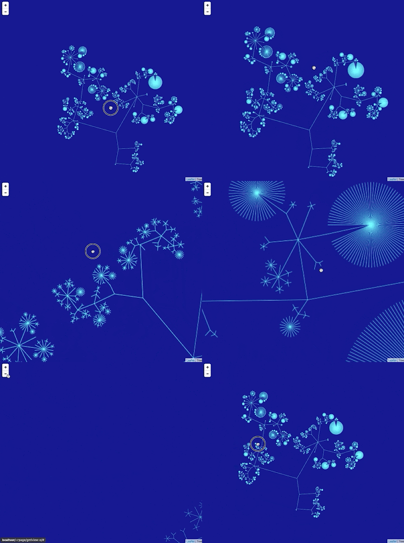
I've created a simple viewer that uses a tiled map viewer (like Google Maps) to display a large graph. The idea is to draw the entire graph scaled to a 256 x 256 pixel tile. The graph is stored in a database that supports geospatial queries, which means the queries to retrieve the individual tiles need to display the graph at different levels of resolution are simply bounding box queries to a database. I realise that this description is cryptic at best. The GitHub repository https://github.com/rdmpage/gml-viewer has more details and the code itself. There's a lot to do, especially adding support for labels(!) which presents some interesting challenges (levels of detail and generalization). The code doesn't do any layout of the graph itself, instead I've used the yEd tool to compute the x,y coordinates of the graph.

Since this exercise was inspired by a discussion of the ASM Mammal Diversity Database, the graph I've used for the demonstration above is the ASM classification of extant mammals. I guess I need to solve the labelling issue fairly quickly!

Maximum entropy summary trees to display higher classifications

How to cite: Page, R. (2021). Maximum entropy summary trees to display higher classifications https://doi.org/10.59350/af01t-6sw74

A challenge in working with large taxonomic classifications is how you display them to the user, especially if the user probably doesn't want all the gory details. For example, the Field Guide app to Victorian Fauna has a nice menu of major animal groups:

This includes both taxonomic and ecological categories (e.g., terrestrial, freshwater, etc.) and greatly simplifies the animal tree of life, but it is a user-friendly way to start browsing a larger database of facts about animals. It would be nice if we could automate constructing such lists, especially for animal groups where the choices of what to display might not seem obvious (everyone wants to see birds, but what insects groups would you prioritise?).

One way to help automate these sort of lists is to use summary trees (see also Karloff, H., & Shirley, K. E. (2013). Maximum Entropy Summary Trees. Computer Graphics Forum, 32(3pt1), 71–80. doi:10.1111/cgf.12094). A summary tree takes a large tree and produces a small summary for k nodes, where k is a number that you supply. In other words, if you want your summary to have 10 nodes then k=10. The diagram below summarises an organisation chart for 43,134 employees.

Summary trees show only a subset of the nodes in the complete tree. All the nodes with a given parent that aren't displayed get aggregated into a newly created "others" node that is attached to that parent. Hence the summary tree alerts the user that there are nodes which list in the full tree but which aren't shown.

Code for maximum entropy summary trees is available in C and R from https://github.com/kshirley/summarytrees, so I've been playing with it a little (I don't normally use R but there was little choice here). As an example I created a simple tree for animals, based on the Catalogue of Life. I took a few phyla and classes and built a tree as a CSV file (see the gist). The file lists each node (uniquely numbered), its parent node (the parent of the root of the tree is "0"), a label, and a weight. For an internal node the weight is always 0, for a leaf the weight can be assigned in various ways. By default you could assign each leaf a weight of 1, but if the "leaf" node represents more than one thing (for example, the class Mammalia) then you can give it the number of species in that class (e.g., 5939). You could also assign weights based on some other measure, such as "popularity". In the gist I got bored and only added species counts for a few taxa, everything else was set to 1.

I then loaded the tree into R and found a summary tree for k=30 (the script is in the gist):

This doesn't look too bad (note as I said above, I didn't fill in all the actual species counts because reasons). If I wanted to convert this into a menu such as the one the Victoria Fauna app uses I would simply list the leaf nodes in order, skipping over those labelled "n others", which would give me:

• Mammalia
• Amphibia
• Reptilia
• Aves
• Actinopterygii
• Hemiptera
• Hymenoptera
• Lepidoptera
• Diptera
• Coleoptera
• Arachnida
• Acanthocephala
• Nemertea
• Rotifera
• Porifera
• Platyhelminthes
• Nematoda
• Mollusca

These 18 taxa are not a bad starting point for a menu, especially if we added pictures from PhyloPic to liven it up. There are probably a couple of animal groups that could be added to make it a bit more inclusive.

Because the technique is automated and fast, it would be straightforward to create submenus for major taxa, with the added advantage that you don't beed to make decisions based whether you know anything about that taxonomic group, it can be driven entirely by species counts (for example). We could also use other measures for weights, such as number of Google search hits, size of pages on Wikipedia, etc. So far I've barely scratched the surface of what could be done with this tool.

P.S. The R code is:

library(devtools)
install_github("kshirley/summarytrees", build_vignettes = TRUE)

library(summarytrees)

data = read.table('/Users/rpage/Development/summarytrees/animals.csv', header=TRUE,sep=",")

g <- greedy(node = data[, "node"], 
            parent = data[, "parent"], 
            weight = data[, "weight"], 
            label = data[, "label"], 
            K = 30)
            write.csv(g$summary.trees[[30]], '/Users/rpage/Development/summarytrees/summary.csv') 

The gist has the data file, and a simple PHP program to convert the output into a dot file to be viewed with GraphViz.

Visualising article coverage in the Biodiversity Heritage Library

It's funny how some images stick in the mind. A few years ago Chris Freeland (@chrisfreeland), then working for Biodiversity Heritage Library (BHL), created a visualisation of BHL content relevant to the African continent. It's a nice example of small multiples.

For more than a decade (gulp) I've been extracting articles from the BHL and storing them in BioStor. My approach is to locate articles based on metadata (e.g., information on title, volume, and pagination) and store the corresponding set of BHL pages in BioStor. BHL in turn regularly harvests this information and displays these articles as "parts" on their web site. Most of this process is semi-automated, but still requires a lot of manual work. One thing I've struggled with is getting a clear sense of how much progress has been made, and how much remains to be done. This has become more pressing given work I'm doing with Nicole Kearney (@nicolekearney) on Australian content. Nicole has a team of volunteers feeding me lists of article metadata for journals relevant to Australian biodiversity, and it would be nice to see where the remaining gaps are.

So, motivated by this, and also a recent comment by Nicky Nicolson (@nickynicolson) about the lack of such visualisations, I've put together a crude tool to try and capture the current state of coverage. You can see the results here: https://rdmpage.github.io/bhl-article-coverage/.

As an example, here is v.25:pt.2 (1988) of Memoirs of the Queensland Museum. Each contiguous block of colour highlights an article in this volume:

This scanned item-level view is constructed for each item (typically a volume or an issue). I then generate a PNG bitmap thumbnail of this display for each volume, and display them together in a page for the corresponding journal (e.g., Memoirs of the Queensland Museum):

So at a glance we can see the coverage for a journal. Gray represents pages that have not been assigned to an article, so if you want to add articles to BHL those are the volumes to focus on.

There's an argument to be made that it is crazy to spend a decade extracting some 226,000 articles semi-automatically. Ideally we could use a tool like machine learning to identify articles in BHL. It would be a huge time saver if we could simply run a BHL article through a tool that could (a) extract article-level metadata and (b) associate that with the corresponding set of scanned pages. Among the possible approaches would be to develop a classifier that would assign each page in a scanned volume to a category such as "article start", "article end", "article", "plate", etc. In effect, we want a tool that can could segment scans into articles (and hence reproduce the coverage diagrams shown above) simply based on attributes of the page images. This doesn't solve the entire problem, we still need to extract metadata (e.g., article titles), but it would be a start. However, it poses the classic dilemma, do I keep doing this manually, or do I stop adding articles and take the time to learn a new technology in the hope that eventually I will end up adding more articles than if I'd persisted with the manual approach?

(by Bruno Oliveir, see Manual tasks of today should be the Automated tasks of tomorrow)

Notes on displaying big trees using Google Maps/Leaflet

Notes to self on web map-style tree viewers. The basic idea is to use Google Maps or Leaflet to display a tree. Hence we need to compute tiles. One approach is to use a database that supports spatial queries to store the x,y coordinates of the tree. When we draw a tile we compute the coordinates of that tile, based on position and zoom level, do a spatial query to extract all lines that intersect with the rectangle for that tile, and draw those.

A nice example of this is Lifemap (see also De Vienne, D. M. (2016). Lifemap: Exploring the Entire Tree of Life. PLOS Biology, 14(12), e2001624. doi:10.1371/journal.pbio.2001624).

It occurs to me that for trees that aren't too big we could do this without an external database. For example, what if we used a Javascript implementation of an R-tree, such as imbcmdth/RTree or its fork leaflet-extras/RTree. So, we could compute the coordinates of the nodes in the tree in "geographic" space, store the bounding box for each line/arc in an R-tree, then query that R-tree for lines that intersect with the bounding box of the relevant tile. We could use a clipping algorithm to only draw the bits of the lines that cross the tile itself.

Web maps, at least in my experience, make trips to a tile server to fetch a tile, we would want instead to call a routine within our web page, because all the data would be loaded into that page. So we'd need to modify the tile creating code.

The ultimate goal would be to have a single page web app that accepts a Newick-style tree and converts into a browsable, zoomable visualisation.

The Semantic Web made fun: d3sparql

Continuing my on-again off-again relationship with the Semantic Web, I stumbled across a cool approach to visualising the results of SPARQL queries. Toshiaki Katayama (@tktym) has put together d3sparql, a set of Javascript scripts that takes SPARQL queries and formats the results graphically using D3.

For example, give the SPARQL endpoint http://togostanza.org/sparql, the following query retrieves the NCBI classification for the tardigrade family Hypsibiidae:

PREFIX rdfs: PREFIX up: SELECT ?root_name ?parent_name ?child_name FROM <http://togogenome.org/graph/uniprot> WHERE { VALUES ?root_name { "Hypsibiidae" } ?root up:scientificName ?root_name . ?child rdfs:subClassOf+ ?root . ?child rdfs:subClassOf ?parent . ?child up:scientificName ?child_name . ?parent up:scientificName ?parent_name . }

By outputting the results as a list of parent-child pairs, it is straightforward to convert the output of this query into a form that D3 accepts, so we can get a tree like this:

The ability to quickly generate trees, charts, and maps from SPARQL queries makes things a lot easier. We can play around a little and explore things. The strength (and challenge) of SPARQL is that it is very open-ended, you can more or less develop queries to do anything. Being able to visualise the results will help guide that exploration.

The code for d3sparql is on GitHub. One "gotcha" is that the cached examples and external Javascript libraries aren't included. I've forked the repository here and added the missing files, so that if you grab that version it works straight out of the box.

Visualising the difference between two taxonomic classifications

It's a nice feeling when work that one did ages ago seems relevant again. Markus Döring has been working on a new backbone classification of all the species which occur in taxonomic checklists harvested by GBIF. After building a new classification the obvious question arises "how does this compare to the previous GBIF classification?" A simple question, answering it however is a little tricky. It's relatively easy to compare two text files -- and this function appears in places such as Wikipedia and GitHub -- but comparing trees is a little trickier. Ordering in trees is less meaningful than in text files, which have a single linear order. In other words, as text strings "(a,b,c)" and "(c,b,a)" are different, but as trees they are the same.

Classifications can be modelled as a particular kind of tree where (unlike, say, phylogenies) every node has a unique label. For example, the tips may be species and the internal nodes may be higher taxa such as genera, families, etc. So, what we need is a way of comparing two rooted, labelled trees and finding the differences. Turns out, this is exactly what Gabriel Valiente and I worked on in this paper doi:10.1186/1471-2105-6-208. The code for that paper (available on GitHub) computes an "edit script" that gives a set of operations to convert one fully labelled tree into another. So I brushed up my rusty C++ skills (I'm using "skills" loosely here) and wrote some code to take two trees and the edit script, and create a simple web page that shows the two trees and their differences. Below is a screen shot showing a comparison between the classification of whales in the Mammals Species of the World, and one from GBIF (you can see a live version here).

The display uses colours to show whether a nodes has been deleted from the first tree, inserted into the second tree, or moved to a different position. Clicking on a node in one tree scrolls the corresponding node in the other tree (if it exists) to scroll into view. Most of the differences between the two trees are due to the absence of fossils from Mammals Species of the World, but there are other issues such as GBIF ignoring tribes, and a few taxa that are duplicated due to spelling typos, etc.

Visualising big phylogenies (yet again)

Inspired in part by the release of the draft tree of life (doi:10.1073/pnas.1423041112 by the Open Tree of Life, I've been revisiting (yet again) ways to visualise very big phylogenies (see Very large phylogeny viewer for my last attempt).

My latest experiment uses Google Maps to render a large tree. Google Maps uses "tiles" to create a zoomable interface, so we need to create tiles for different zoom levels for the phylogeny. To create this visualisation I did the following:

1. The phylogeny laid out in a 256 x 256 grid.
2. The position of each line in the drawing is stored in a MySQL database as a spatial element (in this case a LINESTRING)
3. When the Google Maps interface needs to display a tile at a certain zoom level and location, a spatial SQL query retrieves the lines that intersect the bounds of the tile, then draws those using SVG.

Hence, the tiles are drawn on the fly, rather than stored as images on disk. This is a crude proof of concept so far, there are a few issues to tackle to make this usable:

1. At the moment there are no labels. I would need a way to compute what tables to show at what zoom level ("level of detail"). In other words, at low levels of zoom we want just a few higher taxa to be picked out, whereas as we zoom in we want more and more taxa to be labelled, until at the highest zoom levels we have the tips individually labelled.
2. Ideally each tile would require roughly the same amount of effort to draw. However, at the moment the code is very crude and simply draws every line that intersects a tile. For example, for zoom level 0 the entire tree fits on a single tile, so I draw the entire tree. This is not going to scale to very large trees, so I need to be able to "cull" a lot of the lines and draw only those that will be visible.

In the past I've steered away from Google Maps-style interfaces because the image is zoomed along both the x and y axes, which is not necessarily ideal. But the tradeoff is that I don't have to do any work handling user interactions, I just need to focus on efficiently rendering the image tiles.

All very crude, but I think this approach has potential, especially if the "level of detail" issue can be tackled.

Using GBIF to measure the lag between collection and description of a species (oh dear)

I'm adding more charts to the GBIF Chart tool, including some to explore the type status of specimens from the Solomon Islands. There are nearly 500 holotypes from this region, so quite a few new species have been discovered in this region.

Inspired by the Benoît Fontaine et al. paper on the lag time between a species being discovered and subsequently described (see Species wait 21 years to be described - show me the data) I thought I would do a quick and dirty plot of the difference between the year a specimen was collected and the year the name of the taxon it belongs to was published (from the authorship string for the scientific name). Plotting the results was *cough* interesting:

In theory, the difference between the two dates should be negative (if you subtract publication year from collection year), the smaller number the less the wait for description. But I found some large positive numbers, implying that taxa had been described long before the types were discovered! Something is clearly wrong. What seems to be happening here is the GBIF has failed to match the species name for an occurrence, and so goes up the taxonomic hierarchy and just records the genus. For example, http://gbif.org/occurrence/472764211 was collected in 1965 and is the type of Pandanus guadalcanalius St.John. GBIF doesn't recognise this name, and so matches the occurrence to the genus Pandanus Linnaeus, 1782. hence it looks like we've used a time machine to describe a taxon in 1782 based on a specimen from 1965.

At the other end of the spectrum, there are a lot of specimens that seem to have waited over 200 years for description! Turns out these are mostly specimens from the MCZ that have their collection date recorded by GBIF as "1700-01-01". This seems an arbitrary date, and turns out it's an artefact. The MCZ records "unknown" collection dates as the range 1700-01-01 - 2100-01-01
(see http://mczbase.mcz.harvard.edu/guid/MCZ:IZ:DIPL-4985). Unfortunately, when it generates the export for GBIF, these get truncated to 1700-01-01, and GBIF then (not unreasonably) treats that as the actual collection date. Somewhere in the middle of the plot of lag between collection and description is some interesting information, but it's a pity that most of this is obscured by some serious data errors.

For me the bigger lesson here is the power of visualisation to explore the data and to expose errors. This is why I was underwhelmed by the new charts GBIF is releasing. Plots of ever upward trends are ultimately not very useful. They don't give much insight into the data, nor do they help tackle interesting questions. I think we need a much richer set of visualisations to really understand the strengths and limitations of the data in GBIF.

Update

Investigating further, there are some other reasons for the "back to the future" types. For example, http://www.gbif.org/occurrence/188826624 (CAS 5506 from FishBase) was collected in 1933 and is recorded as a holotype, with the scientific name Cypselurus opisthopus (Bleeker, 1865). 1933 - 1865 = 68, so the taxon was named 68 years before it was collected(!).

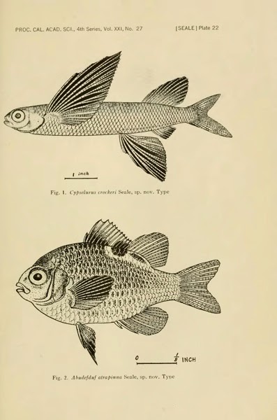
A bit of investigation using BioNames, BioStor, and GBIF (http://www.gbif.org/occurrence/473244692, another record for CAS 5506) reveals that CAS 5506 is the holotype for Cypselurus crockeri, shown below in a plate from it's original description (published in 1935):

Seale A (1935) The Templeton Crocker Expedition to western Polynesian and Melanesian islands, 1933. No. 27. Fishes. Proceedings of the California Academy of Sciences 21: 337–378. http://biostor.org/reference/59326

So, in fact this species was described shortly after its collection, with a lag of 1933 - 1935 = -2 years.


Apart from the duplication issue (FishBase has replicated some of the CAS dataset, sigh), the other problem is one of modelling the data. The CAS record has the original taxon name for which CAS 5506 is the type (Cypselurus crockeri), the FishBase record has the currently accepted name for the taxon (Cypselurus opisthopus). These two different approaches have very different implications for the charts I'm making, and simply reinforce my feeling that the GBIF data is both fascinating and full of "gotchas!".

More on visualisation of GBIF data

Following on from the previous post on visualising GBIF data, I've added some more interactivity. If you click on a pane in the treemap widget you get a list of the corresponding taxa, together with an image from EOL (if one exists). It's a fun way to quickly see what sort of species are present (in this case in the Solomon Islands). You can try it at http://bionames.org/~rpage/gbif-stats/.

Pro tip

It's not obvious from the site, but to go back up the taxonomic hierarchy in the treemap, right click (ctrl-click on a Mac) on the grey bar corresponding to the higher taxon.

Visual analysis of GBIF data

Tim Roberston and the ream at GBIF are working on some nice visualisations of GBIF data, and have made an early release available for viewing: http://analytics.gbif-uat.org. For a given country, say, the Solomon Islands, you can see numerous plots, mostly like this:



Ever the critic, as much as I like this (and appreciate the scale of the task underlying doing analytics on data at the scale of GBIF), what I would really like to see is something that more closely resembles Google Analytics. I want graphs that I can use to get some insight into the data, and which lead me to ask questions (and provide easy for me to discover the answers).

So, I put together a crude, live demo of the sort of thing I'd like to see. You can see it at http://bionames.org/~rpage/gbif-stats (can't promise that this link will be long-lived), and below is a screen shot:

What I've done is fetch all the occurrence records for the Solomon Islands from GBIF (using the API), dumped that into CouchDB, and generated some simple queries. I display the results using Google Charts. There are some similarities with the tools developed by Javier Otegui, Arturo Ariño, and colleagues.

Otegui, J., Ariño, A. H., Encinas, M. A., & Pando, F. (2013, January 25). Assessing the Primary Data Hosted by the Spanish Node of the Global Biodiversity Information Facility (GBIF). (G. P. S. Raghava, Ed.)PLoS ONE. Public Library of Science (PLoS). doi:10.1371/journal.pone.0055144

Otegui, J., & Arino, A. H. (2012, August 15). BIDDSAT: visualizing the content of biodiversity data publishers in the Global Biodiversity Information Facility network. Bioinformatics. Oxford University Press (OUP). doi:10.1093/bioinformatics/bts359

For fun I've also added a map of the GBIF occurrences (also served from CouchDB).

Here's quick guide to some of the charts. Below you can see (left) a plot of species accumulation over time, that is the total number of species that have been collected up to that time. If we had collected all the species we'd expect this to asymptote (flatten out). If it keeps going up, then we still need to do some sampling. On the right is the number of occurrences recorded for each year. You can see that collecting is highly episodic.



To get a little more information on this, I've generated a crude chart where the rows are institutions (e.g., museums and herbaria) that have specimens, and the number of occurrences collected each decade are represented by the shaded boxes (the rightmost box is the current decade) (if you hover over a bar you will see a popup with the decade). To the right is the total number of occurrences.


From this we can see that there have been some major collections at various times (e.g., Kew in the 1960's, the Australian Museum in the 1970's to 1990's). Strangely, the MCZ has lots of specimens from the 1700's, I suspect we have a data quality issue here. There are certainly some issues with dates in this data set, with about a quarter of occurrences with no date:



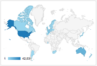
Note that the data for the Solomon Islands, comes from all around the world, mostly from the US. There is a big spike in the date of collection curve in 1944, suggesting a lot of material may be the result of collecting by US servicemen in WW2.



I use a treemap to display the taxonomic distribution of the records, and a donut chart to summarise the taxonomic level to which the occurrences are identified:


The treemap is dominated by vertebrates, which I suspect is a poor reflection of the actual taxonomic composition of the Solomon Islands biota. Over 3/4 of the occurrences are identified to species level, which is encouraging, but there's clearly a lot of material that needs some taxonomic work.

Where next

This has been made in a rush, and there is a lot which could be done. For example, some of the charts would be more useful if you could drill down and explore further. This could be done via the GBIF API or portal (for example, by constructing a URL that shows the portal results for the Solomon Islands for a given year of collection).

There are, of course, issues of scalability. I've made this for the 83,364 occurrences currently in the GBIF portal for the Solomon Islands. There would need to be some thought given to how this could be scaled to larger data sets. But I think this is worth pursuing so that we can get further insights into the remarkable database that GBIF is building.