It's 2023 - why are we still not sharing phylogenies?

How to cite: Page, R. (2023). It’s 2023 - why are we still not sharing phylogenies? https://doi.org/10.59350/n681n-syx67

A quick note to support a recent Twitter thread https://twitter.com/rdmpage/status/1729816558866718796?s=61&t=nM4XCRsGtE7RLYW3MyIpMA

The article “Diversification of flowering plants in space and time” by Dimitrov et al. describes a genus-level phylogeny for 14,244 flowering plant genera. This is a major achievement, and yet neither the tree nor the data supporting that tree are readily available. There is lots of supplementary information (as PDF files), but no machine readable tree or alignment data.

Dimitrov, D., Xu, X., Su, X. et al. Diversification of flowering plants in space and time. Nat Commun 14, 7609 (2023). https://doi.org/10.1038/s41467-023-43396-8

What we have is a link to a web site which in turn has a link to a OneZoom visualisation. If you look at the source code for the web site you can see the phylogeny in Newick format as a Javascript file.

This is a far from ideal way to share data. Readers can’t easily get the tree, explore it, evaluate it, or use it in their own analyses. I grabbed the tree and put it online as a GitHub GIST. Once you have the tree you can do things such as try a different tree viewer, such as PhyloCloud

That is a start, but it’s clearly not ideal. Why didn’t the authors put the tree (and the data) into a proper repository, such as Zenodo where it would be persistent and citable, and also linked to the authors’ ORCID profile? That way everybody wins, readers get a tree to explore, the authors have an additional citable output.

The state of sharing of phylogenetic data is dire, not helped by the slow and painful demise of TreeBASE. Sharing machine readable trees and datasets still does not seem to be the norm in phylogenetics.

Written with StackEdit.

Where are the plant type specimens? Mapping JSTOR Global Plants to GBIF

How to cite: Page, R. (2023). Where are the plant type specimens? Mapping JSTOR Global Plants to GBIF. https://doi.org/10.59350/m59qn-22v52

This blog post documents my attempts to create links between two major resources for plant taxonomy: JSTOR’s Global Plants and GBIF, specifically between type specimens in JSTOR and the corresponding occurrence in GBIF. The TL;DR is that I have tried to map 1,354,861 records for type specimens from JSTOR to the equivalent record in GBIF, and managed to find 903,945 (67%) matches.

Why do this?

Why do this? Partly because a collaborator asked me, but I’ve long been interested in JSTOR’s Global Plants. This was a massive project to digitise plant type specimens all around the world, generating millions of images of herbarium sheets. It also resulted in a standardised way to refer to a specimen, namely its barcode, which comprises the herbarium code and a number (typically padded to eight digits). These barcodes are converted into JSTOR URLs, so that E00279162 becomes https://plants.jstor.org/stable/10.5555/al.ap.specimen.e00279162. These same barcodes have become the basis of efforts to create stable identifiers for plant specimens, for example https://data.rbge.org.uk/herb/E00279162.

JSTOR created an elegant interface to these specimens, complete with links to literature on JSTOR, BHL, and links to taxon pages on GBIF and elsewhere. It also added the ability to comment on individual specimens using Disqus.

However, JSTOR Global Plants is not open. If you click on a thumbnail image of a herbarium sheet you hit a paywall.

In contrast data in GBIF is open. The table below is a simplified comparison of JSTOR and GBIF.

Feature	JSTOR	GBIF
Open or paywall	Paywall	Open
Consistent identifier	Yes	No
Images	All specimens	Some specimens
Types linked to original name	Yes	Sometimes
Community annotation	Yes	No
Can download the data	No	Yes
API	No	Yes

JSTOR offers a consistent identifier (the barcode), an image, has the type linked to the original name, and community annotation. But there is a paywall, and no way to download data. GBIF is open, enables both bulk download and API access, but often lacks images, and as we shall see below, the identifiers for specimens are a hot mess.

The “Types linked to original name” feature concerns whether the type specimen is connected to the appropriate name. A type is (usually) the type specimen for a single taxonomic name. For example, E00279162 is the type for Achasma subterraneum Holttum. This name is now regarded as a synonym of Etlingera subterranea (Holttum) R. M. Sm. following the transfer to the genus Etlingera. But E00279162 is not a type for the name Etlingera subterranea. JSTOR makes this clear by stating that the type is stored under Etlingera subterranea but is the type for Achasma subterraneum. However, this information does not make it to GBIF, which tells us that E00279162 is a type for Etlingera subterranea and that it knows of no type specimens for Achasma subterraneum. Hence querying GBIF for type specimens is potentially fraught with error.

Hence JSTOR has often cleaner and more accurate data. But it is behind a paywall. Hence I set about to get a list of all the type specimens that JSTOR has, and try and match those to GBIF. This would give me a sense of how much content behind JSTOR’s paywall was freely available in GBIF, as well as how much content JSTOR had that was absent from GBIF. I also wanted to use JSTOR’s reference to the original plant name to get around any GBIF’s tendency to link types to the wrong name.

Challenges

Mapping JSTOR barcodes to records in GBIF proved challenging. In an ideal world specimens would have a single identifier that everyone would use when citing or otherwise referring to that specimen. Of course this is not the case. There are all manner of identifiers, ranging from barcodes, collector names and numbers, local database keys (integers, UUIDs, and anything in between). Some identifiers include version codes. All of this greatly complicates linking barcodes to GBIF records. I made extensive use of my Material examined tool that attempts to translate specimen codes into GBIF records. Under the hood this means lots of regular expressions, and I spent a lot of time adding code to handle all the different ways herbaria manage to mangle barcodes.

In some cases JSTOR barcodes are absent from the specimen information in the GBIF occurrence record itself but are hidden in metadata for the image (such as the URL to the image). My “Material examined” tool uses the GBIF API, and that doesn’t enable searches for parts of image URLs. Hence for some herbaria I had to download the archive, extract media URLs and look for barcodes. In the process I encountered a subtle bug in Safari that truncated downloads, see Downloads failing to include all files in the archive.

Some herbaria have data in both JSTOR and GBIF, but no identifiers in common (other than collector names and numbers, which would require approximate string matching). But in some cases the herbaria have their own web sites which mention the JSTOR barcodes, as well as the identifiers those herbaria do share with GBIF. In these cases I would attempt to scrape the herbaria web sites, extract the barcode and original identifier, then find the original identifier in GBIF.

Another observation is that in some cases the imagery in JSTOR is not the same as GBIF. For example LISC002383 and 813346859 are the same specimens but the images are different. Why are the images provided to JSTOR not being provided to GBIF?

In the process of making this mapping it became clear that there are herbaria that aren’t in GBIF, for example Singapore (SING) is not in GBIF but instead is hosted at Oxford University (!) at https://herbaria.plants.ox.ac.uk/bol/sing. There seem to be a number of herbaria that have content in JSTOR but not GBIF, hence GBIF has gaps in its coverage of type specimens.

Interestingly JSTOR rarely seems to be a destination for links. An exception is the Paris museum, for example specimens MPU015018 has a link to JSTOR record for same specimen MPU015018.

Matching taxonomic names

As a check on matching JSTOR to GBIF I would also check that the taxonomic names associated with the two records are the same. The challenge here is that the names may have changed. Ideally both JSTOR and GBIF would have either a history of name changes, or at least the original name the specimen was associated with (i.e., the name for which the specimen is the type). And of course, this isn’t the case. So I relied on a series of name comparisons, such as “are the names the same?”, “if names are different are the specific epithets the same?”, and “if names are specific epithets are different are the generic names the same?”. Because the spelling of species names can change depending on the gender of the genus, I also used some stemming rules to catch names that were the same even if their ending was different.

This approach will still miss some matches, such as hybrid names, and cases where a specimen is stored under a completely different name (e.g., the original name is a heterotypic synonym of a different name).

Mapping

The mapping made so far is available on GitHub https://github.com/rdmpage/jstor-plant-specimens and Zenodo https://doi.org/10.5281/zenodo.10044359.

At the time of writing I have retrieved 1,354,861 records for type specimens from JSTOR, of which 903,945 (67%) have been matched to GBIF.

This has been a sobering lesson in just how far we are from being able to treat specimens as citable things, we simply don’t have decent identifiers for them. JSTOR made a lot of progress, but that has been hampered by being behind a paywall, and the fact that many of these identifiers are being lost or mangled by the time they make their way into GBIF, which is arguably where most people get information on specimens.

There’s an argument that it would be great to get JSTOR Global Plants into GBIF. It would certainly add a lot of extra images, and also provide a presence for a number of smaller herbaria that aren’t in GBIF. I think there’s also a case to be made for having a GBIF hosted portal for plant type specimens, to help make these valuable objects more visible and discoverable.

Below is a barchart of the top 50 herbaria ranked by number of type specimens in JSTOR, showing the numbers of specimens mapped to GBIF (red) and those not found (blue).

Reading

• Boyle, B., Hopkins, N., Lu, Z. et al. The taxonomic name resolution service: an online tool for automated standardization of plant names. BMC Bioinformatics 14, 16 (2013). https://doi.org/10.1186/1471-2105-14-16

• CETAF Stable Identifiers (CSI)

• CETAF Specimen URI Tester

• Holttum, R. E. (1950). The Zingiberaceae of the Malay Peninsula. Gardens’ Bulletin, Singapore, 13(1), 1-249. https://biostor.org/reference/163926

• Hyam, R.D., Drinkwater, R.E. & Harris, D.J. Stable citations for herbarium specimens on the internet: an illustration from a taxonomic revision of Duboscia (Malvaceae) Phytotaxa 73: 17–30 (2012). https://doi.org/10.11646/phytotaxa.73.1.4

• Rees T (2014) Taxamatch, an Algorithm for Near (‘Fuzzy’) Matching of Scientific Names in Taxonomic Databases. PLoS ONE 9(9): e107510. https://doi.org/10.1371/journal.pone.0107510

• Ryan D (2018) Global Plants: A Model of International Collaboration . Biodiversity Information Science and Standards 2: e28233. https://doi.org/10.3897/biss.2.28233

• Ryan, D. (2013), THE GLOBAL PLANTS INITIATIVE CELEBRATES ITS ACHIEVEMENTS AND PLANS FOR THE FUTURE. Taxon, 62: 417-418. https://doi.org/10.12705/622.26

• (2016), Global Plants Sustainability: The Past, The Present and The Future. Taxon, 65: 1465-1466. https://doi.org/10.12705/656.38

• Smith, G.F. and Figueiredo, E. (2013), Type specimens online: What is available, what is not, and how to proceed; Reflections based on an analysis of the images of type specimens of southern African Polygala (Polygalaceae) accessible on the worldwide web. Taxon, 62: 801-806. https://doi.org/10.12705/624.5

• Smith, R. M. (1986). New combinations in Etlingera Giseke (Zingiberaceae). Notes from the Royal Botanic Garden Edinburgh, 43(2), 243-254.

• Anna Svensson; Global Plants and Digital Letters: Epistemological Implications of Digitising the Directors’ Correspondence at the Royal Botanic Gardens, Kew. Environmental Humanities 1 May 2015; 6 (1): 73–102. doi: https://doi.org/10.1215/22011919-3615907

Written with StackEdit.

Document layout analysis

How to cite: Page, R. (2023). Document layout analysis. https://doi.org/10.59350/z574z-dcw92

Some notes to self on document layout analysis.

I’m revisiting the problem of taking a PDF or a scanned document and determining its structure (for example, where is the title, abstract, bibliography, where are the figures and their captions, etc.). There are lots of papers on this topic, and lots of tools. I want something that I can use to process both born-digital PDFs and scanned documents, such as the ABBYY, DjVu and hOCR files on the Internet Archive. PDFs remain the dominant vehicle for publishing taxonomic papers, and aren’t going away any time soon (see Pettifer et al. for a nuanced discussion of PDFs).

There are at least three approaches to document layout analysis.

Rule-based

The simplest approach is to come up rules, such as “if the text is large and it’s on the first page, it’s the title of the article”. Examples of more sophisticated rules are given in Klampfl et al., Ramakrishnan et al., and Lin. Rule-based methods can get you a long way, as shown by projects such as Plazi. But there are always exceptions to rules, and so the rules need constant tweaking. At some point it makes sense to consider probabilistic methods that allow for uncertainty, and which can also “learn”.

Large language models (LLMs)

At the other extreme are Large language models (LLMs), which have got a lot of publicity lately. There are a number of tools that use LLMs to help extract information from documents, such as LayoutLM (Xu et al.), Layout Parser, and VILA (Shen et al.). These approaches encode information about a document (in some case including the (x,y) coordinates of individual words on a page) and try and infer which category each word (or block of text) belongs to. These methods are typically coded in Python, and come with various tools to display regions on pages. I’ve had variable success getting these tools to work (I am new to Python, and am also working on a recent Mac which is not the most widely used hardware for machine learning). I have got other ML tools to work, such as an Inception-based model to classify images (see Adventures in machine learning: iNaturalist, DNA barcodes, and Lepidoptera), but I’ve not succeeded in training these models. There are obscure Python error messages, some involving Hugging Face, and eventually my patience wore out.

Another aspect of these methods is that they often package everything together, such that they take a PDF, use OCR or ML methods such as Detectron to locate blocks, then encode the results and feed them to a model. This is great, but I don’t necessarily want the whole package, I want just some parts of it. Nor does the prospect of lengthy training appeal (even if I could get it to work properly).

The approach that appealed the most is VILA, which doesn’t use (x,y) coordinates directly but instead encodes information about “blocks” into text extracted from a PDF, then uses an LLM to infer document structure. There is a simple demo at Hugging Face. After some experimentation with the code, I’ve ended up using the way VILA represents a document (a JSON file with a series of pages, each with lists of words, their positions, and information on lines, blocks, etc.) as the format for my experiments. If nothing else this means that if I go back to trying to train these models I will have data already prepared in an appropriate format. I’ve also decided to follow VILA’s scheme for labelling words and blocks in a document:

• Title
• Author
• Abstract
• Keywords
• Section
• Paragraph
• List
• Bibliography
• Equation
• Algorithm
• Figure
• Table
• Caption
• Header
• Footer
• Footnote

I’ve tweaked this slightly by adding two additional tags
from VILA’s Labeling Category Reference, the “semantic” tags “Affiliation” and “Venue”. This helps separate information on author names (“Author”) from their affiliations, which can appear in very different positions to the author’s names. “Venue” is useful to label things such as a banner at the top of an article where the publisher display the name of the journal, etc.

Conditional random fields

In between masses of regular expressions and large language models are approaches such as Conditional random fields (CRFs), which I’ve used before to parse citations (see Citation parsing tool released). Well known tools such as GROBID use this approach.

CRFs are fast, and somewhat comprehensible. But it does require Feature engineering, that is, you need to come up with features of the data to help train the model (for the systematists among you, this is very like coming up with characters for a bunch of taxa). This is were you can reuse the rules developed in a rules-based approach, but instead of having the rules make decisions (e.g., “big text = Title”), you just a rule that detects whether text is big or not, and the model combined with training data then figures out if and when big text means “Title”. So you end up spending time trying to figure out how to represent document structure, and what features help the model get the right answer. For example, methods such as Lin’s for detecting whether there are recurring elements in a document are great source of features to help recognise headers and footers. CRFs also make it straightforward to include dependencies (the “conditional” in the name). For example, a bibliography in a paper can be recognised not just by a line having a year in it (e.g., “2020”), but there being nearby lines that also have years in them. This helps us avoid labelling isolated lines with years as “Bibliography” when they are simply text in a paragraph that mentions a year.

Compared to LLMs this a lot of work. In principle with an LLM you “just” take a lot of training data (e.g., text and location on a page) and let the model to the hard work of figuring out which bit of the document corresponds to which category (e.g., title, abstract, paragraph, bibliography). The underlying model has already been trained on (potentially) vast amounts of text (and sometimes also word coordinates). But on the plus side, training CRFs is very quick, and hence you can experiment with adding or removing features, adding training data, etc. For example, I’ve started training with about ten (10) documents, training takes seconds, and I’ve got serviceable results.

Lots of room for improvement, but there’s a constant feedback loop of seeing improvements, and thinking about how to tweak the features. It also encourages me to think about what went wrong.

Problems with PDF parsing

To process PDFs, especially “born digital” PDFs I rely on pdf2xml, originally written by Hervé Déjean (Xerox Research Centre Europe). It works really well, but I’ve encountered a few issues. Some can be fixed by adding more fonts to my laptop (from XpdfReader), but others are more subtle.

The algorithm used to assign words to “blocks” (e.g., paragraphs) seems to struggle with superscripts (e.g., ¹), which often end up being treated as separate blocks. This breaks up lines of text, and also makes it harder to accurately label parts of the document such as “Author” or “Affiliation”.

Figures can also be problematic. Many are simply bitmaps embedded in a PDF and can be easily extracted, but sometimes labelling on those bitmaps, or indeed big chunks of vector diagrams are treated as text, so we end up with story text blocks in odd positions. I need to spend a little time thinking about this as well. I also need to understand the “vet” format pdftoxml extracts from PDFs.

PDFs also have all sorts of quirks, such as publishers slapping cover pages on the front, which make feature engineering hard (the biggest text might now be not be the title but some cruff from the publisher). Sometimes there are clues in the PDF that it has been moodier.! For example, ResearchGate inserts a “rgid” tag in the PDF when it adds a cover page.

Yes but why?

So, why I am doing this? Why battle with the much maligned PDF format. It’s because a huge chunk of taxonomic and other information is locked up in PDFs, and I’d like a simpler, scalable, way to extract some of that. Plazi is obviously the leader in this are in terms of the amount of information they have extracted, but their approach is labour-intensive. I want something that is essentially automatic, that can be trained to handle the idiosyncracities of the taxonomic literature, and can be applied to both born digital PDFs and OCR from scans in the Biodiversity Heritage Library and elsewhere. Even if we could simply extract bibliographic information (to flesh out the citation graph) and the figures, that would be progress.

References

Déjean H, Meunier J-L (2006) A System for Converting PDF Documents into Structured XML Format. In: Bunke H, Spitz AL (eds) Document Analysis Systems VII. Springer, Berlin, Heidelberg, pp 129–140 https://doi.org/10.1007/11669487_12

Klampfl S, Granitzer M, Jack K, Kern R (2014) Unsupervised document structure analysis of digital scientific articles. Int J Digit Libr 14(3):83–99. https://doi.org/10.1007/s00799-014-0115-1

Lin X (2003) Header and footer extraction by page association. In: Document Recognition and Retrieval X. SPIE, pp 164–171 https://doi.org/10.1117/12.472833

Pettifer S, McDERMOTT P, Marsh J, Thorne D, Villeger A, Attwood TK (2011) Ceci n’est pas un hamburger: modelling and representing the scholarly article. Learned Publishing 24(3):207–220. https://doi.org/10.1087/20110309

Ramakrishnan C, Patnia A, Hovy E, Burns GA (2012) Layout-aware text extraction from full-text PDF of scientific articles. Source Code for Biology and Medicine 7(1):7. https://doi.org/10.1186/1751-0473-7-7

Shen Z, Lo K, Wang LL, Kuehl B, Weld DS, Downey D (2022) VILA: Improving Structured Content Extraction from Scientific PDFs Using Visual Layout Groups. Transactions of the Association for Computational Linguistics 10:376–392. https://doi.org/10.1162/tacl_a_00466

Xu Y, Li M, Cui L, Huang S, Wei F, Zhou M (2020) LayoutLM: Pre-training of Text and Layout for Document Image Understanding. In: Proceedings of the 26th ACM SIGKDD International Conference on Knowledge Discovery & Data Mining. pp 1192–1200

Written with StackEdit.

The problem with GBIF's Phylogeny Explorer

How to cite: Page, R. (2023). The problem with GBIF’s Phylogeny Explorer. https://doi.org/10.59350/v0bt3-zp114

GBIF recently released the Phylogeny Explorer, using legumes as an example dataset. The goal is to enables users to “view occurrence data from the GBIF network aligned to legume phylogeny.” The screenshot below shows the legume phylogeny side-by-side with GBIF data.

Now, I’m all in favour of integrating phylogenies and occurrence data, and I have a lot of respect for the people behind this project (Morten Høfft and Thomas Stjernegaard Jeppesen), but I think this way of displaying a phylogeny has multiple problems. Indeed, it suffers from many of the classic “mistakes” people make when trying to view big trees.

Why maps work

Tree visualisation is a challenging problem. I wrote a somwhwat out of date review on this topic a decade ago, and Googling will find many papers on the topic. There is also the amazing treevis.net.

I think the key issues can be seen once we compare the tree on the left with the map on the right. The map allows zooming in and out, and it does this equally in both the x and y dimensions. In other words, when you zoom in the map expands left to right and top to bottom. This makes sense because the map is a square. Obviously the Earth is not a square, but the projection used by web maps (such as Google Maps, OpenStreetMap, etc.) treats the world as one. Below is the world at zoom level 0, a 256 x 256 pixel square.

When you zoom in the number of tiles is doubled with each increase in zoom level, and you get a more and more detailed map. As you zoom in on a map typically you see labels appearing and disappearing. These labels are (a) always legible, and (b) they change with zoom level. Continent names appear before cities, but disappear once you’ve zoomed in to country level or below.

To summarise, the map visualisation zooms appropriately, always has legible labels, and the level of detail and labelling changes with zoom level. None of this is true for the GBIF phylogeny viewer.

The phylogeny problem

The screenshot below shows GBIF’s display of the legume tree such that the whole tree fits into the window. No labels are visible, and the tree structure is hard to see. There are no labels for major groups, so we have no obvious way to find our way around the tree.

We can zoom so that we can see the labels, but everything is zoomed, such that we can’t see all the tree structure to the left.

Indeed, if we zoom in more we rapidly lose sight of most of the tree.

This is one of the challenges presented by trees. Like space, they are mostly empty. hence simply zooming in is often not helpful.

So, the zooming doesn’t correspond to the structure of the tree, labels are often either not legible or absent, and levels of detail don’t change with zooming in and out.

What can we do differently?

I’m going to sketch an alternative approach to viewing trees like this. I have some ropey code that I’ve used to create the diagrams below. This isn’t ready for prime time, but hopefully illustrates the idea. The key concept is that we zoom NOT by simply expanding the viewing area in the x and y direction, but by collapsing and expanding the tree. Each zoom level corresponds the number of nodes we will show in the tree. We use a criterion to rank the importance of each node in the tree. One approach is how “distinctive” the nodes are, see Jin et al. 2009. We then use a priority queue to chose the nodes to display at a given zoom level (see Libin et al. 2017 and Zaslavsky et al. 2007).

Arguably this gives us a more natural way to zoom a tree, we see the main structure first, then as we zoom in more structure becomes apparent. It turns out if the tree drawing itself is constructed using a “in-order” traversal we can greatly simplify the drawing. Imagine that the tree consists of a number of nodes (both internal and external, i.e., leaves and hypothetical ancestors), and we draw each node on a single line (as if we were using a line printer). Collapsing or expanding the tree is simply a matter of removing or adding lines. If a node is not visible we don’t draw it. If a leaf node is visible we show it as if the whole tree was visible. Internal nodes are slightly different. If it is visible but collapsed we can draw it with a triangle representing the descendants, if it is not collapsed then we draw it as if the whole tree was visible. The end result is that we don’t need to recompute the tree as we zoom in or out, we simply compute which nodes to show, and in what state.

As an experiment I decided to explore the legume tree used in the GBIF website. As is sadly so typical, the original publication of the tree (Ringelberg et al. 2023) doesn’t provide the actual tree, but I found a JSON version on GitHub https://github.com/gbif/hp-legume/tree/master/assets/phylotree. I then converted that to Newick format so my tools could use it (had a few bumpy moments when I discovered that the tree has negative branch lengths!). The converted file is here: https://gist.github.com/rdmpage/ef43ea75a738e75ec303602f76bf0b2e

I then ran the tree through my code and generated views at various zoom levels.

Note that as the tree expands labels are always legible, and zooming only increased the size of the tree in the y-axis (as the expanded nodes take up more space). Note also that we see a number of isolated taxa appearing, such as Lachesiodendron viridiflorum. These taxa are often of evolutionary interest, and also of high conservation interest due to their phylogenetic isolation. Simply showing the whole tree hides these taxa.

Now, looking at these two diagrams there are two obvious limitations. The first is that the black triangles representing collapsed clades are all the same size regardless of whether they represent a few of many taxa. This could be addressed by adding numbers beside each triangle, using colour to reflect the numebr of collapsed nodes, or perhaps by breaking the “one node per row” rule by drawing particularly large nodes over two or more lines.

The other issue is that most of the triangles lack labels. This is because the tree itself lacks them (I added “Ingoid clade”, for example). There will be lots of nodes which can be labelled (e.g., by genus name), but once we start displaying phylogeny we will need to make use of informal names, or construct labels based on the descendants (e.g., “genus 1 - genus 5”). We can also think of having sets of labels that we locate on the tree by finding the least common ancestor (AKA the most recent common ancestor) of that label (hello Phylocode).

Another consideration is what to do with labels as taxa are expanded?. One approach would be to use shaded regions, for example in the last tree above we could shade the clades rooted at Mimosa, Vachellia, and the “Ingoid clade” (and others if they had labels). If we were clever we could alter which clades are shaded based on the zoom level. If we wanted these regions to not overlap (for example, if we wanted bands of colour corresponding to clades to appear on the right of the tree) then we could use something like maximum disjoint sets to choice the best combination of labels.

Summary

I don’t claim that this alternative visualisation is perfect (and my implementation of it is very far from perfect). but I think it shows that there are ways we can zoom into trees that reflects tree structure, ensures labels are always legible, and that supports levels of detail (collapsed nodes expanding as we zoom). The use of inorder traversal and three styles of node drawing mean that the diagram is simple to render. We don’t need fancy graphics, we can simply have a list of images.

To conclude, I think it’s great GBIF is moving to include phylogenies. But we can't visualise phylogeny as a static image, it's a structure that requires us to think about how to display it with the same level of creativity that makes web maps such a successful visualisation.

Reading

Jin Chen, MacEachren, A. M., & Peuquet, D. J. (2009). Constructing Overview + Detail Dendrogram-Matrix Views. IEEE Transactions on Visualization and Computer Graphics, 15(6), 889–896. https://doi.org/10.1109/tvcg.2009.130

Libin, P., Vanden Eynden, E., Incardona, F., Nowé, A., Bezenchek, A., … Sönnerborg, A. (2017). PhyloGeoTool: interactively exploring large phylogenies in an epidemiological context. Bioinformatics, 33(24), 3993–3995. doi:10.1093/bioinformatics/btx535

Page, R. D. M. (2012). Space, time, form: Viewing the Tree of Life. Trends in Ecology & Evolution, 27(2), 113–120. https://doi.org/10.1016/j.tree.2011.12.002)

Ribeiro, P. G., Luckow, M., Lewis, G. P., Simon, M. F., Cardoso, D., De Souza, É. R., Conceição Silva, A. P., Jesus, M. C., Dos Santos, F. A. R., Azevedo, V., & De Queiroz, L. P. (2018). lachesiodendron , a new monospecific genus segregated from piptadenia(Leguminosae: Caesalpinioideae: mimosoid clade): evidence from morphology and molecules. TAXON, 67(1), 37–54. https://doi.org/10.12705/671.3

Ringelberg, J. J., Koenen, E. J. M., Sauter, B., Aebli, A., Rando, J. G., Iganci, J. R., De Queiroz, L. P., Murphy, D. J., Gaudeul, M., Bruneau, A., Luckow, M., Lewis, G. P., Miller, J. T., Simon, M. F., Jordão, L. S. B., Morales, M., Bailey, C. D., Nageswara-Rao, M., Nicholls, J. A., … Hughes, C. E. (2023). Precipitation is the main axis of tropical plant phylogenetic turnover across space and time. Science Advances, 9(7), eade4954. https://doi.org/10.1126/sciadv.ade4954

Zaslavsky L., Bao Y., Tatusova T.A. (2007) An Adaptive Resolution Tree Visualization of Large Influenza Virus Sequence Datasets. In: Măndoiu I., Zelikovsky A. (eds) Bioinformatics Research and Applications. ISBRA 2007. Lecture Notes in Computer Science, vol 4463. Springer, Berlin, Heidelberg. https://doi.org/10.1007/978-3-540-72031-7_18

Written with StackEdit.

Sub-second searching of millions of DNA barcodes using a vector database

How to cite: Page, R. (2023). Sub-second searching of millions of DNA barcodes using a vector database. https://doi.org/10.59350/qkn8x-mgz20

Recently I’ve been messing about with DNA barcodes. I’m junior author with David Schindel on forthcoming book chapter Creating Virtuous Cycles for DNA Barcoding: A Case Study in Science Innovation, Entrepreneurship, and Diplomacy, and I’ve blogged about Adventures in machine learning: iNaturalist, DNA barcodes, and Lepidoptera. One thing I’ve always wanted is a simple way to explore DNA barcodes both geographically and phylogenetically. I’ve made various toys (e.g., Notes on next steps for the million DNA barcodes map and DNA barcode browser) but one big challenge has been search.

The goal is to be able to do is take a DNA sequence and search the DNA barcode database for barcodes that are similar to that sequence, then build a phylogenetic tree for the results. And I want this to be fast. The approach I used in my :“DNA barcode browser” was to use Elasticsearch and index the DNA sequences as n-grams (=k-mers). This worked well for small numbers of sequences, but when I tried this for millions of sequences things got very slow, typically it took around eight seconds for a search to complete. This is about the same as BLAST on my laptop for the same dataset. These sort of search times are simply too slow, hence I put this work on the back burner. That is, until I started exploring vector databvases.

Vector databases, as the name suggests, store vectors, that is, arrays of numbers. Many of the AI sites currently gaining attention use vector databases. For example, chat bots based on ChatGPT are typically taking text, converting it to an “embedding” (a vector), then searching in a database for similar vectors which, hopefully, correspond to documents that are related to the original query (see ChatGPT, semantic search, and knowledge graphs).

The key step is to convert the thing you are interested in (e.g., text, or an image) into an embedding, which is a vector of fixed length that encodes information about the thing. In the case of DNA sequences one way to do this is to use k-mers. These are short, overlapping fragments of the DNA sequence (see This is what phylodiversity looks like). In the case of k-mers of length 5 the embedding is a vector of the frequencies of the 4⁵ = 1,024 different k-mers for the letters A, C, G, and T.

But what do we do with these vectors? This is where the vector database comes in. Search in a vector database is essentially a nearest-neighbour search - we want to find vectors that are similar to our query vector. There has been a lot of cool research on this problem (which is now highly topical because of the burgeoning interest in machine learning), and not only are there vector databases, but tools to add this functionality to existing databases.

So, I decided to experiment. I grabbed a copy of PostgreSQL (not a database I’d used before), added the pgvector extension, then created a database with over 9 million DNA barcodes. After a bit of faffing around, I got it to work (code still needs cleaning up, but I will release something soon).

So far the results are surprisingly good. If I enter a nucleotide sequence, such as JF491468 (Neacomys sp. BOLD:AAA7034 voucher ROM 118791) and search for the 100 most similar sequences I get back 100 Neacomys sequences in 0.14 seconds(!). I can then take the vectors for each of those sequences (i.e., the array of k-mer frequencies), compute a pairwise distance matrix, then build a phylogeny (in PAUP,* naturally).

Searches this rapid mean we can start to interactively explore large databases of DNA barcodes, as well as quickly take new, unknown sequences and ask “have we seen this before?”

As a general tool this approach has limitations. Vector databases have a limit on the size of vector they can handle, so k-mers much larger than 5 will not be feasible (unless the vectors are sparse in the sense that not all k-mers actually occur). Also it’s not clear to me how much this approach succeeds because of the nature of barcode data. Typically barcodes are either very similar to each other (i.e., from the same species), or they are quite different (the famous “barcode gap”). This may have implications for the success of nearest neighbour searching.

Still early days, but so far this has been a revelation, and opens up some interesting possibilities for how we could explore and interact with DNA barcodes.

Written with StackEdit.

What, if anything, is the Biodiversity Knowledge Hub?

How to cite: Page, R. (2023). What, if anything, is the Biodiversity Knowledge Hub? https://doi.org/10.59350/axeqb-q2w27

To much fanfare BiCIKL launched the “Biodiversity Knowledge Hub” (see Biodiversity Knowledge Hub is online!!!). This is advertised as a “game-changer in scientific research”. The snappy video in the launch tweet claims that the hub will

• it will help your research thanks to interlinked data…
• …and responds to complex queries with the services provided…

Interlinked data, complex queries, this all sounds very impressive. The video invites us to “Vist the Biodiversity Knowledge Hub and give it a shot”. So I did.

The first thing that strikes me is the following:

Disclaimer: The partner Organisations and Research Infrastructures are fully responsible for the provision and maintenance of services they present through BKH. All enquiries about a particular service should be sent directly to its provider.

If the organisation trumpeting a new tool takes no responsibility for that tool, then that is a red flag. To me it implies that they are not taking this seriously, they have no skin in the game. If this work mattered you’d have a vested interest in seeing that it actually worked.

I then tried to make sense of what the Hub is an what it offers.

Is it maybe an aggregation? Imagine diversity biodiversity datasets linked together in a single place so that we could seamlessly query across that data, bouncing from taxa to sequences to ecology and more. GBIF and GenBank are examples of aggregations here data is brought together, cleaned, reconciled, and services built on top of that. You can go to GBIF and get distribution data for a species, you can go to GenBank and compare your sequence with millions of others. Is the Hub an aggregation?.. no, it is not.

Is it afederation? Maybe instead of merging data from multiple sources, that data lives on the original sites, but we can query across it a bit like a travel search engine queries across multiple airlines to find us the best flight. The data still needs to be reconciled, or at least share identifiers and vocabularies. Is the Hub a federation?.. no, it is not.

OK, so maybe we still have data in separate silos, but maybe the Hub is a data catalogue where we can search for data using text terms (a bit like Google’s Dataset Search)? Or even better, maybe it describes the data in machine readable terms so that we could find out what data are relevant to our interests (e.g., what data sets deal with taxa and ecological associations base don sequence data?). Is it a data catalogue? … no, it is not.

OK, then what actually is it?

It is a list. They built a list. If you go to FAIR DATA PLACE you see an invitation to EXPLORE LINKED DATA. Sounds inviting (“linked data, oohhh”) but it’s a list of a few projects: ChecklistBank, e-Biodiv, LifeBlock, OpenBiodiv, PlutoF, Biodiversity PMC, Biotic Interactions Browser, SIBiLS SPARQL Endpoint, Synospecies, and TreatmentBank.

These are not in any way connected, they all have distinct APIs, different query endpoints, speak different languages (e.g., REST, SPARQL), and there’s no indication that they share identifiers even if they overlap in content. How can I query across these? How can I determine whether any of these are relevant to my interests? What is the point in providing SPARQL endpoints (e.g., OpenBiodiv, SIBiLS, Synospecies) without giving the user any clue as to what they contain, what vocabularies they use, what identifiers, etc.?

The overall impression is of a bunch of tools with varying levels of sophistication stuck together on a web page. This is in no way a “game-changer”, nor is it “interlinked data”, nor is there any indication of how it supports “complex queries”.

It feels very much like the sort of thing one cobbles together as a demo when applying for funding. “Look at all these disconnected resources we have, give us money and we can join them together”. Instead it is being promoted as an actual product.

Instead of the hyperbole, why not tackle the real challenges here? At a minimum we need to know how each service describes data, those services should use the same vocabularies and identifiers for the same things, be able to tell us what entities and relationships they cover, and we should be able to query across them. This all involves hard work, obviously, so let’s stop pretending that it doesn’t and do that work, rather than claim that a list of web sites is a “game-changer”.

Written with StackEdit.

Adventures in machine learning: iNaturalist, DNA barcodes, and Lepidoptera

How to cite: Page, R. (2023). Adventures in machine learning: iNaturalist, DNA barcodes, and Lepidoptera. https://doi.org/10.59350/5q854-j4s23

Recently I’ve been working with a masters student, Maja Nagler, on a project using machine learning to identify images of Lepidoptera. This has been something of an adventure as I am new to machine learning, and have only minimal experience with the Python programming language. So what could possibly go wrong?

The inspiration for this project comes from (a) using iNaturalist’s machine learning to help identify pictures I take using their app, and (b) exploring DNA barcoding data which has a wealth of images of specimens linked to DNA sequences (see gallery in GBIF), and presumably reliably identified (by the barcodes). So, could we use the DNA images to build models to identify specimens? Is it possible to use models already trained on citizen science data, or do we need custom models trained on specimens? Can models trained on museum specimens be used to identify living specimens?

To answer this we’ve started simple, using the iNaturalist 2018 competition as a starting point. There is a code in GitHub for an entry in that challenge, and the challenge data is available, so the idea was to take that code and model and see how well it works on DNA barcode images.

That was the plan. I ran into a slew of Python-related issues involving out of date code, dependencies, and issues with running on a MacBook. Python is, well, a mess. I know there are ways to “tame” the mess, but I’m amazed that anyone can get anything done in machine learning given how temperamental the tools are.

Another consideration is that machine learning is computationally intensive, and typically uses PC with NVIDIA chips. Macs don 't have these chips. However, Apple’s newer Macs provide Metal Performance Shaders (MPS) which does speed things up. But getting everything to work together was a nightmare. This is a field full of obscure incantations, bugs, and fixes. I describe some of the things I went through in the README for the repository. Note that this code is really a safety net. Maja is working on a more recent model (using Google’s Colab), I just wanted to make sure that we had a backup in place in case my notion that this ML stuff would be “easy” turned out to be, um, wrong.

Long story short, everything now works. Because our focus is Lepidoptera (moths and butterflies) I ended up subsetting the original challenge dataset to include just those taxa. This resulted in 1234 species. This is obviously a small number, but it means we can train a reasonable model in less than a week (ML is really, really, computationally expensive).

There is still lots to do, but I want to share a small result. After training the model on Lepidoptera from the iNaturalist 2018 dataset, I ran a small number of images from the DNA barcode dataset. The results are encouraging. For example, for Junonia villida all the barcoded specimens were either correctly identified (green) or were in the top three hits (orange) (the code works is it outputs the top three hits for each image). So a model trained on citizen science images of (mostly) living specimens can identify museum specimens.

For other species the results are not so great, but are still interesting. For example, for Junonia orithya quite a few images are not correctly identified (red). Looking at the images, it looks like specimens photographed ventrally are going to be a problem (unlikely to be common angle for photographs of living specimens), and specimens with scale grids and QR codes are unlikely to be seen in the wild(!).

An obvious thing to do would be to train a model based on DNA barcode specimens and see how well it identifies citizen science images (and Maja will be doing just that). If that works well, then that would suggest that there is scope for expanding models for identifying live insects to include museum specimen images (and visa versa), see also Towards a digital natural history museum.

It is early days, still lots of work to do, and deadlines are pressing, but I’m looking forward to seeing how Maja’s project evolves. Perhaps the pain of Python, PyTorch, MPS, etc. will all be worth it.

Written with StackEdit.

A taxonomic search engine

How to cite: Page, R. (2023). A taxonomic search engine. https://doi.org/10.59350/r3g44-d5s15

Tony Rees commented on my recent post Ten years and a million links. I’ve responded to some of his comments, but I think the bigger question deserves more space, hence this blog post.

Tony’s comment

Hi Rod, I like what you’re doing. Still struggling (a little) to find the exact point where it answers the questions that are my “entry points” so to speak, which (paraphrasing a post of yours from some years back) start with:

• Is this a name that “we” (the human race I suppose) recognise as having been used for a taxon (think Global Names Resolver, Taxamatch, etc.) - preferably an automatable query and response (i.e., a machine can ask it and incorporated the result into a workflow)
• Does it refer to a currently accepted taxon or if not, what is the accepted equivalent
• What is its taxonomic placement (according to one or a range of expert systems)
• Also, for reporting/comparison/analysis purposes…
  - How many accepted taxa (at whatever rank) are currently known in group X (or the whole world)
• How many new names (accepted or unaccepted) were published in year A (or date range A-C)
• How many new names were published (or co-authored) by author Z
• (and probably more)

Having access to more of the primary literature is great, and necessary, but does not help me in those respects (since the published works must still be parsed by a human, not a machine). But maybe it does answer some other questions like how many original works were published by author Z, in a particular time frame.

Of course as you will be aware, using ORCIDs for authors is only a small portion of the puzzle, since ORCIDs are not issued for deceased authors, or those who never request one, so far as I am aware.

None of the above is a criticism of what you are doing! Just trying to see if I can establish any new linkages to what you are doing which will enable me to automate portions of my own efforts to a greater degree (let machines do things that currently still require a human). So far (as evidenced by the most recent ION data dump you were able to supply) it is giving me a DOI in many cases as a supplement to the title of the original work (per ION/Zoological Record) which is something of a time saver in my quest to read the original work (from which I could extract the DOI as well once reached) but does not really automate anything since I still have to try and find it in order to peruse the content.

Mostly random thoughts above, possibly of no use, but I do ruminate on the universe of connected “things not strings” in the hope that one day life will get easier for biodiversity informatics workers, or maybe that the “book of life” will be self-assembling…

My response

I think there are several ways to approach this. I’ll walk through them below, but TL;DR

• Define the questions we have and how we would get the answers. For example, what combination database and SQL queries, or web site and API calls, or knowledge graph and SPARQL do we need to answer each question?
• Decide what sort of interface(s) we want. Do we want a web site with a search box, a bunch of API calls, or a natural language interface?
• If we want natural language, how do we do that? Do we want a ChatBot?
• And as an aside, how can we speed up reading the taxonomic literature?

The following are more notes than a reasoned essay. I wanted to record a bunch of things to help me think about these topics.

Build a natural language search engine

One of the first things I read that opened my eyes to the potential of OpenAI-powered tools and how to build them was Paul Graham GPT which I talked about here. This is a simple question and answer tool that takes a question and returns an answer, based on Paul Graham’s blog posts. We could do something similar for taxonomic names (or indeed, anything where we have some text and want to query it). At its core we have a bunch of blocks of text, embeddings for those blocks, then we get embeddings for the question and find the best-matching embeddings for the blocks of text.

Generating queries

One approach is to use ChatGPT to formulate a database query based on a natural langue question. There have been a bunch of people exploring generating SPARQL queries from natural langue, e.g. ChatGPT for Information Retrieval from Knowledge Graph, ChatGPT Exercises — Generating a Course Description Knowledge Graph using RDF, and Wikidata and ChatGPT and this could be explored for other query languages.

So in this approach we take natural language questions and get back the queries we need to answer those questions. We then go away and run those queries.

Generating answers

This still leaves us with what to do with the answers. Given, say, a SPARQL response, we could have code that generates a bunch of simple sentences from that response, e.g. “name x is a synonym of name y”, “there are ten species in genus x”, “name x was published in the paper zzz”, etc. We then pass those sentences to an AI to summarise into nicer natural language. We should aim for something like the Wikipedia-derived snippets from DBpedia (see Ozymandias meets Wikipedia, with notes on natural language generation). Indeed, we could help make more engaging answers by adding DBpedia snippets for the relevant taxa, abstracts from relevant papers, etc. to the SPARQL results and ask the AI to summarise all of that.

Skipping queries altogether

Another approach is to generate all the answers ahead of time. Essentially, we take our database or knowledge graph and generate simplified sentences summarising everything we know: “species x was described by author y in 1920”, “species x was synonymies with species y in 1967”, etc. We then get embeddings for these answers, store them in a vector database, and we can query them using a chatbot-style interface.

There is a big literature on embedding RDF (see RDF2vec.org), and also converting RDF to sentences. These “RDF verbalisers” are further discussed on the WebNLG Challenge pages, and an example is here: jsRealB - A JavaScript Bilingual Text Realizer for Web Development.

This approach is like the game Jeopardy!: we generate all the answers and the goal is to match the user’s question to one or more of those answers.

Machine readability

Having access to more of the primary literature is great, and necessary, but does not help me in those respects (since the published works must still be parsed by a human, not a machine).

This is a good point, but help is at hand. There are a bunch of AI tools to “read” the literature for you, such as SciSpace’s Copilot. I think there’s a lot we could do to explore these tools. We could also couple them with the name - publication links in the ten year library. For example, if we know that there is a link between a name and a DOI, and we have the text for the article with that DOI we could then ask targeted questions regarding what the papers says about that name. One way to implement this is to do something similar to the Paul Graham GPT demo described above. We take the text of the paper, chunk it into smaller blocks (e.g., paragraphs), get embeddings for each block, add those to a vector database, and we can then search that paper (and others) using natural language. We could imagine an API that takes a paper and splits out the core “facts” or assertions that the paper makes. This also speaks to Notes on collections, knowledge graphs, and Semantic Web browsers where I bemoaned the lack of a semantic web browser.

Summary

I think the questions being asked are all relatively straightforward to answer, we just need to think a little bit about the best way to answer them. Much of what I’ve written above is focussed on making such a system more broadly useful and engaging, with richer answers that a simple database query. But a first step is to define the questions and the queries that would answer them, then figure out what interface to wrap this up in.

Written with StackEdit.

Ten years and a million links

As trailed on a Twitter thread last week I’ve been working on a manuscript describing the efforts to map taxonomic names to their original descriptions in the taxonomic literature.

Putting together a manuscript on linking taxonomic names to the primary literature, basically “um, what, exactly, have you been doing all these years?”. TL;DR Across fungi, plants, and animals approx 1.3 million names have been linked to a persistent identifier for a publication.

— Roderic Page (@rdmpage) May 25, 2023

The preprint is on bioRxiv doi:10.1101/2023.05.29.542697

A major gap in the biodiversity knowledge graph is a connection between taxonomic names and the taxonomic literature. While both names and publications often have persistent identifiers (PIDs), such as Life Science Identifiers (LSIDs) or Digital Object Identifiers (DOIs), LSIDs for names are rarely linked to DOIs for publications. This article describes efforts to make those connections across three large taxonomic databases: Index Fungorum, International Plant Names Index (IPNI), and the Index of Organism Names (ION). Over a million names have been matched to DOIs or other persistent identifiers for taxonomic publications. This represents approximately 36% of names for which publication data is available. The mappings between LSIDs and publication PIDs are made available through ChecklistBank. Applications of this mapping are discussed, including a web app to locate the citation of a taxonomic name, and a knowledge graph that uses data on researcher’s ORCID ids to connect taxonomic names and publications to authors of those names.

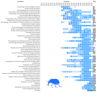
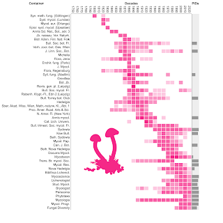
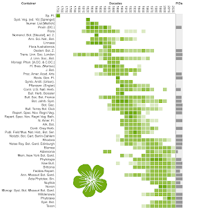
Much of the work has been linking taxa to names, which still has huge gaps. There are also interesting differences in coverage between plants, animals, and fungi (see preprint for details).

There is also a simple app to demonstrate these links, see https://species-cite.herokuapp.com.

Written with StackEdit.

Library interfaces, knowledge graphs, and Miller columns

Some quick notes on interface ideas for digital libraries and/or knowledge graphs.

Recently there’s been something of an explosion in bibliographic tools to explore the literature. Examples include:

• Elicit which uses AI to search for and summarise papers
• _scite which uses AI to do sentiment analysis on citations (does paper A cite paper B favourably or not?)
• ResearchRabbit which uses lists, networks, and timelines to discover related research
• Scispace which navigates connections between papers, authors, topics, etc., and provides AI summaries.

As an aside, I think these (and similar tools) are a great example of how bibliographic data such as abstracts, the citation graph and - to a lesser extent - full text - have become commodities. That is, what was once proprietary information is now free to anyone, which in turns means a whole ecosystem of new tools can emerge. If I was clever I’d be building a Wardley map to explore this. Note that a decade or so ago reference managers like Zotero were made possible by publishers exposing basic bibliographic data on their articles. As we move to open citations we are seeing the next generation of tools.

Back to my main topic. As usual, rather than focus on what these tools do I’m more interested in how they look. I have history here, when the iPad came out I was intrigued by the possibilities it offered for displaying academic articles, as discussed here, here, here, here, and here. ResearchRabbit looks like this:

Scispace’s “trace” view looks like this:

What is interesting about both is that they display content from left to right in vertical columns, rather than the more common horizontal rows. This sort of display is sometimes called Miller columns or a cascading list.

By Gürkan Sengün (talk) - Own work, Public Domain, https://commons.wikimedia.org/w/index.php?curid=594715

I’ve always found displaying a knowledge graph to be a challenge, as discussed elsewhere on this blog and in my paper on Ozymandias. Miller columns enable one to drill down in increasing depth, but it doesn’t need to be a tree, it can be a path within a network. What I like about ResearchRabbit and the original Scispace interface is that they present the current item together with a list of possible connections (e.g., authors, citations) that you can drill down on. Clicking on these will result in a new column being appended to the right, with a view (typically a list) of the next candidates to visit. In graph terms, these are adjacent nodes to the original item. The clickable badges on each item can be thought of as sets of edges that have the same label (e.g., “authored by”, “cites”, “funded”, “is about”, etc.). Each of these nodes itself becomes a starting point for further exploration. Note that the original starting point isn’t privileged, other than being the starting point. That is, each time we drill down we are seeing the same type of information displayed in the same way. Note also that the navigation can be though of as a card for a node, with buttons grouping the adjacent nodes. When we click on an individual button, it expands into a list in the next column. This can be thought of as a preview for each adjacent node. Clicking on an element in the list generates a new card (we are viewing a single node) and we get another set of buttons corresponding to the adjacent nodes.

One important behaviour in a Miller column interface is that the current path can be pruned at any point. If we go back (i.e., scroll to the left) and click on another tab on an item, everything downstream of that item (i.e., to the right) gets deleted and replaced by a new set of nodes. This could make retrieving a particular history of browsing a bit tricky, but encourages exploration. Both Scispace and ResearchRabbit have the ability to add items to a collection, so you can keep track of things you discover.

Lots of food for thought, I’m assuming that there is some user interface/experience research on Miller columns. One thing to remember is that Miller columns are most often associated with trees, but in this case we are exploring a network. That means that potentially there is no limit to the number of columns being generated as we wander through the graph. It will be interesting to think about what the average depth is likely to be, in other words, how deep down the rabbit hole will be go?

Update

Should add link to David Regev's explorations of Flow Browser.

Written with StackEdit.

ChatGPT, semantic search, and knowledge graphs

One thing about ChatGPT is it has opened my eyes to some concepts I was dimly aware of but am only now beginning to fully appreciate. ChatGPT enables you ask it questions, but the answers depend on what ChatGPT “knows”. As several people have noted, what would be even better is to be able to run ChatGPT on your own content. Indeed, ChatGPT itself now supports this using plugins.

Paul Graham GPT

However, it’s still useful to see how to add ChatGPT functionality to your own content from scratch. A nice example of this is Paul Graham GPT by Mckay Wrigley. Mckay Wrigley took essays by Paul Graham (a well known venture capitalist) and built a question and answer tool very like ChatGPT.

Because you can send a block of text to ChatGPT (as part of the prompt) you can get ChatGPT to summarise or transform that information, or answer questions based on that information. But there is a limit to how much information you can pack into a prompt. You can’t put all of Paul Graham’s essays into a prompt for example. So a solution is to do some preprocessing. For example, given a question such as “How do I start a startup?” we could first find the essays that are most relevant to this question, then use them to create a prompt for ChatGPT. A quick and dirty way to do this is simply do a text search over the essays and take the top hits. But we aren’t searching for words, we are searching for answers to a question. The essay with the best answer might not include the phrase “How do I start a startup?”.

Semantic search

Enter Semantic search. The key concept behind semantic search is that we are looking for documents with similar meaning, not just similarity of text. One approach to this is to represent documents by “embeddings”, that is, a vector of numbers that encapsulate features of the document. Documents with similar vectors are potentially related. In semantic search we take the query (e.g., “How do I start a startup?”), compute its embedding, then search among the documents for those with similar embeddings.

To create Paul Graham GPT Mckay Wrigley did the following. First he sent each essay to the OpenAI API underlying ChatGPT, and in return he got the embedding for that essay (a vector of 1536 numbers). Each embedding was stored in a database (Mckay uses Postgres with pgvector). When a user enters a query such as “How do I start a startup?” that query is also sent to the OpenAI API to retrieve its embedding vector. Then we query the database of embeddings for Paul Graham’s essays and take the top five hits. These hits are, one hopes, the most likely to contain relevant answers. The original question and the most similar essays are then bundled up and sent to ChatGPT which then synthesises an answer. See his GitHub repo for more details. Note that we are still using ChatGPT, but on a set of documents it doesn’t already have.

Knowledge graphs

I’m a fan of knowledge graphs, but they are not terribly easy to use. For example, I built a knowledge graph of Australian animals Ozymandias that contains a wealth of information on taxa, publications, and people, wrapped up in a web site. If you want to learn more you need to figure out how to write queries in SPARQL, which is not fun. Maybe we could use ChatGPT to write the SPARQL queries for us, but it would be much more fun to be simply ask natural language queries (e.g., “who are the experts on Australian ants?”). I made some naïve notes on these ideas Possible project: natural language queries, or answering “how many species are there?” and Ozymandias meets Wikipedia, with notes on natural language generation.

Of course, this is a well known problem. Tools such as RDF2vec can take RDF from a knowledge graph and create embeddings which could in tern be used to support semantic search. But it seems to me that we could simply this process a bit by making use of ChatGPT.

Firstly we would generate natural language statements from the knowledge graph (e.g., “species x belongs to genus y and was described in z”, “this paper on ants was authored by x”, etc.) that cover the basic questions we expect people to ask. We then get embeddings for these (e.g., using OpenAI). We then have an interface where people can ask a question (“is species x a valid species?”, “who has published on ants”, etc.), we get the embedding for that question, retrieve natural language statements that the closest in embedding “space”, package everything up and ask ChatGPT to summarise the answer.

The trick, of course, is to figure out how t generate natural language statements from the knowledge graph (which amounts to deciding what paths to traverse in the knowledge graph, and how to write those paths is something approximating English). We also want to know something about the sorts of questions people are likely to ask so that we have a reasonable chance of having the answers (for example, are people going to ask about individual species, or questions about summary statistics such as numbers of species in a genus, etc.).

What makes this attractive is that it seems a straightforward way to go from a largely academic exercise (build a knowledge graph) to something potentially useful (a question and answer machine). Imagine if something like the defunct BBC wildlife site (see Blue Planet II, the BBC, and the Semantic Web: a tale of lessons forgotten and opportunities lost) revived here had a question and answer interface where we could ask questions rather than passively browse.

Summary

I have so much more to learn, and need to think about ways to incorporate semantic search and ChatGPT-like tools into knowledge graphs.

Written with StackEdit.

ChatGPT, of course

I haven’t blogged for a while, work and other reasons have meant I’ve not had much time to think, and mostly I blog to help me think.

ChatGPT is obviously a big thing at the moment, and once we get past the moral panic (“students can pass exams using AI!”) there are a lot of interesting possibilities to explore. Inspired by essays such as How Q&A systems based on large language models (eg GPT4) will change things if they become the dominant search paradigm — 9 implications for libraries and Cheating is All You Need, as well as [Paul Graham GPT](https://paul-graham-gpt.vercel.app) I thought I’d try a few things and see where this goes.

ChatGPT can do some surprising things.

Parse bibliographic data

I spend a LOT of time working with bibliographic data, trying to parse it into structured data. ChatGPT can do this:

Note that it does more than simply parse the strings, it expands journal abbreviations such as “J. Malay Brch. R. Asiat. Soc.” to the full name “Journal of the Malayan Branch of the Royal Asiatic Society”. So we can get clean, parsed data in a range of formats.

Parse specimens

Based on the success with parsing bibliographic strings I wondered how well it could handle citation software specimens (“material examined”). Elsewhere I’ve been critical of Plazi’s ability to do this, see Problems with Plazi parsing: how reliable are automated methods for extracting specimens from the literature?.

For example, given this specimen record on p. 130 of doi:10.5852/ejt.2021.775.1553

LAOS • Kammoune Province, Bunghona Market, 7 km Nof Xe Bangfai River;
17.13674° N, 104.98591° E; E. Jeratthitikul, K. Wisittikoson, A. Fanka, N. Wutthituntisil and P. Prasankok leg.; sold by local people;
MUMNH-UNI2831.

ChatGPT extracted a plausible Darwin Core record:

I’ve been experimenting with parsing specimen records using the same machine learning approach for bibliographic data (e.g., Citation parsing tool released), perhaps it’s time to rethink that idea.

Correct OCR errors

OCR errors are a well known limitation of the Biodiversity Heritage Library (BHL), see for example OCR Improvements: An Early Analysis. Given that ChatGPT is built on top of a large language model it seems obvious to see how it handles OCR errors. I tried the following snippet of text from BHL page 4312227:

i BREVIORA No. 185

Jiiaii Jr., 16, who always join him and Hedriek in th(> search for
frogs. Iloraeio Mayorga, research assistant to tlie author, has also
been (wtreniely useful, not only in field work, but also in the
tedious curatorial and laboratory work that usually fol- lows. Dr.
John Randall kindly took tlie photouraplis of E. hedricki, and the
Galiiiaues family of San Juan made their El Verde house available as
a (MMiter of activities for the colleetiuff party. To all these
jx’opic, the autlioi- feels (iee])ly indebted.

Elet’tiierodactylus iiKnRrcKi s]). n.

Type. Museum of Coniparative Zoology Xo. ;}()!)()8, c^ from El Verde,
west flank of El Yuiuinc Puerto Hico. I.IOO ft. Coll. J. A. Kivero,
11 Aug-. I!)(i2.

ChatGPT returns this:

i BREVIORA No. 185

Juan Jr., 16, who always joins him and Hedrick in the search for
frogs. Horacio Mayorga, research assistant to the author, has also
been extremely useful, not only in field work, but also in the tedious
curatorial and laboratory work that usually follows. Dr. John Randall
kindly took the photographs of E. hedricki, and the Galinanes family
of San Juan made their El Verde house available as a center of
activities for the collecting party. To all these people, the author
feels deeply indebted.

Eleutherodactylus hedricki sp. n.

Type. Museum of Comparative Zoology No. 30908, c? from El Verde, west
flank of El Yunque, Puerto Rico. 1100 ft. Coll. J. A. Rivero, 11 Aug.
1962.

Comparing this to the scanned image ChatGPT it does pretty well, for example the gobbledegook “Elet’tiierodactylus iiKnRrcKi” is correctly translated as “Eleutherodactylus hedricki”. Running all of BHL through ChatGPT probably isn’t feasible, but one could imagine targeted cleaning of key papers.

Summary

These small experiments are fairly trivial, but they are the sort of tedious tasks that would otherwise require significant programming (or other resources) to solve. But ChatGPT can do rather more, as I hope to discuss in the next post.

Written with StackEdit.